Cross validating your machine learning models
There is a common trope about data science that beginner data scientists often outperform more experienced ones and get models with 99,9% accuracy, compared to experienced data scientists, who rarely get 80%. Yet, as the term implies, data science is all about data and science. And science means having a good validation protocol.
Cross Validation Strategies
Learning is a process that involves:
Gathering data
Making a model or hypothesis that explains the experimental data
Checking that hypothesis on never-seen data _(See this excellent, if very technical article, about learning by Scott Aaronson .)
Like human learning, machine learning should follow this protocol. Most scientists are fully aware of how important the third part of the process is, because building models that work only on the data you got is not very useful. But for those just starting out in data science, it’s a common mistake to neglect it.
Often, ignoring this step results in models that get very high performances while experimenting, but then collapse when deployed and used on real, never beforeseen data. This comes from two main phenomena:
Data overfitting
Data leakage

A poorly done modelization. Model scored 88,976 RMSE on training data, but a 346,703 RMSE on validation data.
As machine learning is very powerful, data overfitting can, and will, happen a lot. With thousands of parameters, you will always succeed in building a model that perfectly fits your experimental data, yet predicts few — or no — new data.
Another issue, data leakage, is when your model starts to memorize the relationship between samples and targets instead of understanding them. It’s common with data that’s split into groups, like categories of goods or people. The model might memorize the group’s most frequent target instead of the relationship between its feature and the target.
When confronted with a new category of goods, the model will then be clueless.
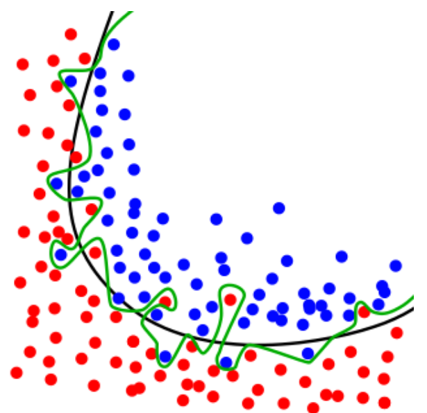
A 100% accurate model, in green, and a good model, in black.
Validation technique: Know about the future performance
Validation techniques are an important part of a solid strategy in order to keep models and hyperparameters performing their best on future data.
It’s a set of techniques that helps guarantee that, in addition to getting a good model initially, the model will stay good when exposed to new data. In other words, the wonderful performance you got in the lab won’t collapse when your company agrees to use your model worldwide for piloting all its vital processes.
Common techniques to prevent performance collapse
Luckily, the validation problem has been widely studied and we, as data scientists, benefit from several methods to get model performance as good in production as it was during experimentation. All of these methods rely on a common principle — put data aside when training, and evaluate models on the data put aside.
Yet, the art is all about knowing which data to put aside.
Level 0: Train test split
The first technique is a very basic one, but it works: Get our data, split it in two sets, usually 80% and 20% of the size of the original dataset, respectively called the trainset and holdout. Then, train on one set, and measure performance on the other one.

Even if it’s not foolproof, this technique often prevents too much overfitting and is the least time-consuming. Split your data, make one train pass,and validate! Just be sure to use a sample without replacement when splitting your dataset, so none of the sample data in the trainset is memorized and then automatically predicted during validation (except if you want to cheat).
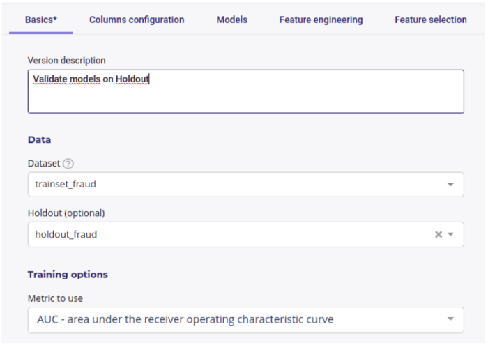
Use two datasets: One for training, one for validation.
Level 0.5: Train test split with good normalization
Before moving on to the next technique, let’s talk about a common error that’s often underestimated. Data scientists frequently normalize, or apply some kind of transformation, to data before training. When doing that, always fit your transformation on the trainset, not the whole dataset.
cheat).
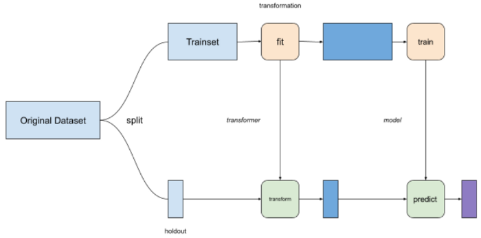
Do
If you apply some kind of transformation, like normalization, to the whole dataset, some information will leak between the holdout step to the training step. You will get a little boost of performance from it, but that boost will disappear when the model goes into production.
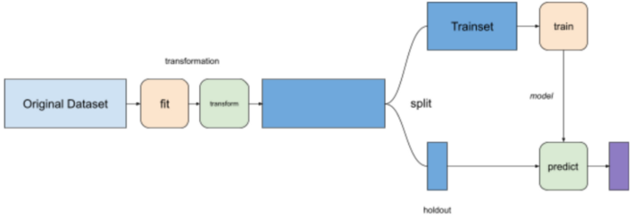
Don’t
Level 1: Folds
In the very basic technique of splitting a dataset, we did not address the topic of variance, or stability, of a model.

Variance represented as error bar on each model performance.
Variance is a way to quantify how much your performance will change if you change the split of your model, even if you preserve the underlying distribution across each trial.
It is a very good indicator of generalization capability, as your performance should not change that much if you randomly sample training data from your original dataset.
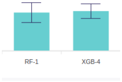
Which one would you put to real use? RF-1 is a little bit better, but if you take its standard deviation into consideration, represented as an error bar, expect to be less confident about its performance on future data.
If the performance changes significantly when you change your training data, it means that the way you built your model is very unstable and, in most cases, it will be very unpredictable when put in production.
It’s like reaching a high equilibrium on top of a very narrow mountain. You get to be the best, but any minor change in the data could throw everything off and plummet you to the bottom.
That’s why when building models, you should adopt a K-fold validation strategy:
Choose an integer k (generally k = 3 or 5 works well).
Split your dataset into k parts.
Choose one part.
Train on the remaining (k-1) parts.
Validate on the part you chose in step 3.
Start again from step 3, until you round around all of your k parts.
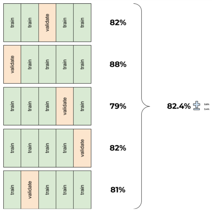
By splitting data in a round robin manner you got two results: - Average performance - Variance of this performance
There is no definitive way to solve the tradeoff of performance vs. variance, but as a data scientist, you must be aware of the consequences of selecting a high-variance model — and be able to explain that to your business coworkers.
In the Prevision.io platform, k-fold cross-validation is always done each time a model is trained, and variance is displayed on the model list of each version, so you can choose which one fits best with your team. (Or, more precisely, Prevision.io’s platform uses a stratified k-fold strategy — check it out in the next section.)

Don’t feel that good about this one…
Level 2: Stratify
Even when folding, another problem would arise when the data is very unbalanced.
Let’s say that you are training a classifier on a dataset whose target rate is 1%, and you use a 5-fold strategy. On a dataset of 100,000, each fold will be 20,000 samples, and the training set on each round will be 80,000 samples. As the target rate is 1%, we expect to get 800 positives in the training set and 200 in the validation set.
Yet, if you just sample randomly, the distribution of your target rate will look this way.
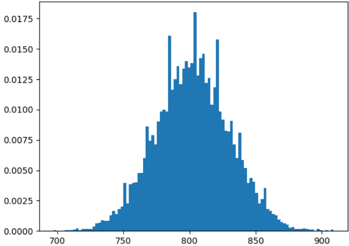
In approximately 10% of your folding round, the target rate difference between the trainset and the validation set will be more than 10%!
In the worst case, for example, your trainset could get 720 out of 1,000 of the existing positives,that is a 0.9% rate, while the validation set would get 280 positives, a 1,4% rate.
This Problem only increases with lower target rates. With a target rate of 0.1%, you can see a 10x factor between the target rate of the trainset and the validation set when splitting your fold with a basic random algorithm. One of the most common use cases where this problem arises is in building a fraud classifier, as it’s very common that fraud target rates are low.
Cross-validating data with this method is a bad practice as the performance and variance you gain are built on poor foundations. Expecting consistent and reliable performance is not possible.
In order to avoid this, you need to use a stratified k-fold cross-validation strategy, which is a way of splitting the data so that the trainset and validation set always have the same target rate. Even on a balanced dataset, the impact of a stratified k-fold is clearly visible compared to a simple k-fold split:
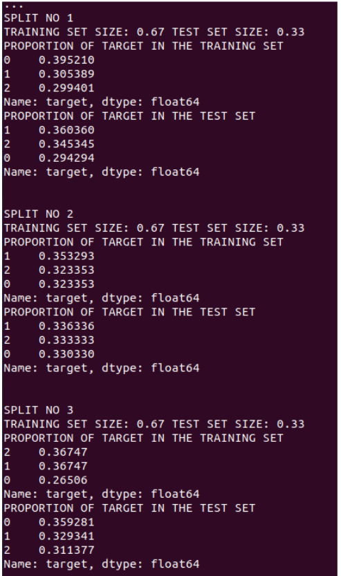
k-fold
To a stratified one where target rate is well distributed across folds :
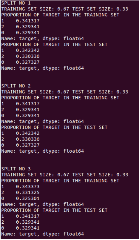
stratified k-fold
Level 3: Custom Folds
The last common technique, and a very important one, solves the problems that arise on two types of datasets:
Dataset with time-indexed data
Dataset with columns that represent some kind of group, like goods or people
With this kind of data, machine learning models sometimes get some information from future leakage, or group leakage, and instead of deducing general rules about the relationship between the features and target, it memorizes the average target value of a group or a period of time.
Let’s say, for example, that you want to build a model that predicts the prices that customers are willing to pay for fruits based on some of their features (e.g. weight, amount of sugar, origin, or color).
One of your columns probably is the category of fruit (apple, berries, etc.).
If you build a model that uses the category of fruit as a feature, you will probably get some good results. BUT, if a new kind of fruit comes in, your model will probably fail because instead of really learning what determined the price of a fruit, it instead memorized your existing catalog. So sometimes you need to build custom folds in order to know how your model will behave when a new item from an unknown category comes in. Custom folds depend entirely on your use case, and should be built manually with regards to the problem you want to solve in the context of your application .
Temporal data presents the same kind of trap. If you use just a random fold across your dataset, you’re going to leak some data from the future that you cannot expect to benefit from when applying the model in real usage.
For example, if you build a trainset with some data from each year over a 10-year span, your model will probably learn some target statistics from each year. For example, if in 2020 the average price of a fruit is 2,3€, you cannot use that for a year that hasn’t happened yet, e.g. 2023.
What you really want are general rules that stay true in the future, e.g. a price increase of 3% each year since 2000, or something like that.
Even if using stratified k-fold, you should not sample random data across the whole dataset, but instead build a new feature, often called “fold” that respects the unknown in your future data.
In the case of a fruit category, you could attribute an integer to each category of fruit and split your data regarding this number. In other words:
Train model on banana and apples, validate it on citrus
Train model on citrus and apples, validate on banana
Train model on banana and citrus, validate on apple
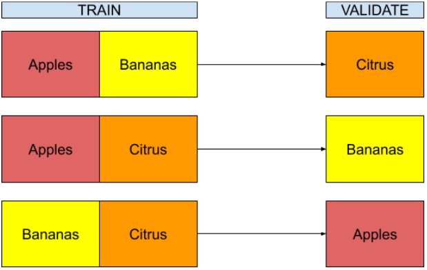
The performance will probably decline from building folds this way, but you could expect it to stay stable if your grocery gets a new kind of fruit.
For temporal data, in addition to folding over a component of the date (year, month, week), you should train on past data and validate on future data. This strategy is called temporal blocks folding and should always be used when dealing with temporal data. It might look like:
Training on 2010 and 2011, validating on 2012
Training on 2010, 2011 and 2012, validating on 2013
Training on 2010, 2011, 2012, 2013 through 2019, validating on 2020
These cross-validation strategies, both group folding and temporal block folding, are quite complex and you really need to understand your data well to implement them. Because building custom folds always leads to a dip in performance, you want to be sure that doing so serves a model stability purpose.
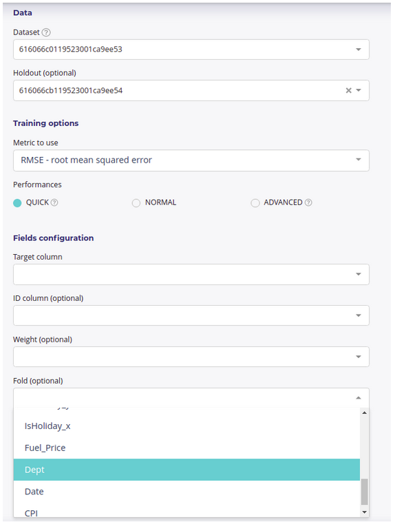
In the Prevision.io platform, you could define one of your columns as a custom fold and the cross-validation will be done along that fold. When you use the “timeseries” training type, the platform will automatically use a temporal block to compute its cross-validation score, so you don’t need to define blocks by yourself.
The impact of a cross-validation strategy
Let’s see how a cross-validation strategy may impact your performance.
We built a dataset of sales, with two categories (product and date/time), ranging over 3 years, and decided to measure the performance by holding out sales from 2012 and training models on sales from 2010 and 2011. The quality of our models will be measured as the RMSE on holdout, and we used 6 different folding strategies:

No folds: We don’t input any folds, so Prevision.io will just use a random stratified k-fold along the trainset
Random folds: We use a 7-fold, built randomly
Trimester folds: Trimesters (4) are used as fold
All month folds: Months (12) are used as fold
Triplet month folds: The month number modulo 3 is used as fold (e.g, we train on January and February, and validate on March)
Store folds: We use the store number as fold
Results
Here is a summary of the model’s performance for each strategy. Remember, the lower the RMSE, the better.
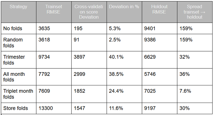
We see that there are 3 main types of input from our strategy:
Strategies with no smart folds get very good models (no folds and random rolds) in the trainset, as their RMSE are the best. But when applied on holdout, the performance totally collapses. You should never use models like that.
Some models (rimester folds and ll month folds) get the worst score, but remain more stable, and we get a similar performance in holdout. Yet the variance in cross-validation, and the fact that the holdout score is lower than the trainset score, must trigger attention. These models should probably be tested on more data to validate their stability or lack of stability.
The triplet month fold strategy gets some good performance on the trainset and a very similar one on the holdout. The variance of cross-validation is still high, but could probably be lowered with more powerful models. Of the three, this fold strategy is probably the strongest, and more powerful modelisation algorithm could now be used to get better performance
Note that folding on the store columns get some interesting results, but this is probably due to the lack of temporal folds, which artificially decrease the RMSE and improve their performance.