Synthetic Data for machine Learning : A guide
As often quoted, “Data is the new oil” and we, datascientist, clearly know the value of good data to train our model. However, we often face some problems with datas :
we don’t have access them because of confidentiality issues
we do not have enough
they are unbalanced and thus lead to biased model toward more represented class.
In this guide, we discuss the usage and performance of synthetic data generation. If you want to try it by yourself you can :
Grab the dataset in our datapack section
generate Fake data with our synthetic data generation datascience service
Usage of synthetic Data
A common problem in B2C industry, telecom, bank,… And healthcare is confidentiality of data. We want to build models upon some dataset but want to avoid showing any information about personal record.
For example, you may have a dataset whom each rows is age, gender, size, weight, place of residence,… Even if data are anonymized by removing name or email, it’s often easy to find some particular person which unique combination of features, for example :
A 30 years old man who live near Gare du nord, earn 30 000€ a month , whom wife is engineer and had subscribed to sport magazine
would be unique enough to know a lot about him, even without identity data. So for some industry, exposing suche sensitive data, even for modeling, is clearly a no go.
Second problem is lack of data or worst, lack of data for some segment of the population that will then be disadvantaged by models.
For example, let’s say that we got a dataset with 10000 men and 1000 womens and we are using RMSE as Metric for our training. Let’s say for sake of this article that every prediction for man have the same error \(manError\) and womens have a \(womanError\) constant error
The Score of a model will be :
df['RMSE'] = ((10000*(df['manError']**2) + 1000*(df['womanError']**2))/(10000 + 1000))**.5
And the errors of each gender will weight as follows on the training metric :
FemaleError |
100 |
200 |
1000 |
2000 |
10000 |
100000 |
MaleError |
||||||
100 |
100.0 |
112 |
316 |
610 |
3016 |
30151 |
200 |
193 |
200.0 |
356 |
632 |
3021 |
30151 |
1000 |
953 |
955 |
1000 |
1128 |
3162 |
30166 |
2000 |
1907 |
1907 |
1930 |
2000.0 |
3567 |
30211 |
10000 |
9534 |
9534 |
9539 |
9553 |
10000 |
31622 |
100000 |
95346 |
95346 |
95346 |
95348 |
95393 |
100000 |
We clearly see that making an error on woman segment weights much less on the optimized metric, as going from a \(100\) to \(10000\) woman error only goes from \(100\) to \(3016\) total error yet for man it goes from \(100\) to \(9534\).
As goal of machine learning model are to find minimum of givne metrics, a model trained on this data will advantage man Segment over woman Segment. Of course, if we had the same number of mens datas and womens datas, the error will be balanced and no bias toward some segment will happen. But adding more woman datas is not enough, we cannot just copy and paste more rows, as it will lack of diversity.
What we should do instead is adding “realistic” woman Datas by sampling from the underlying distribution of each woman feature
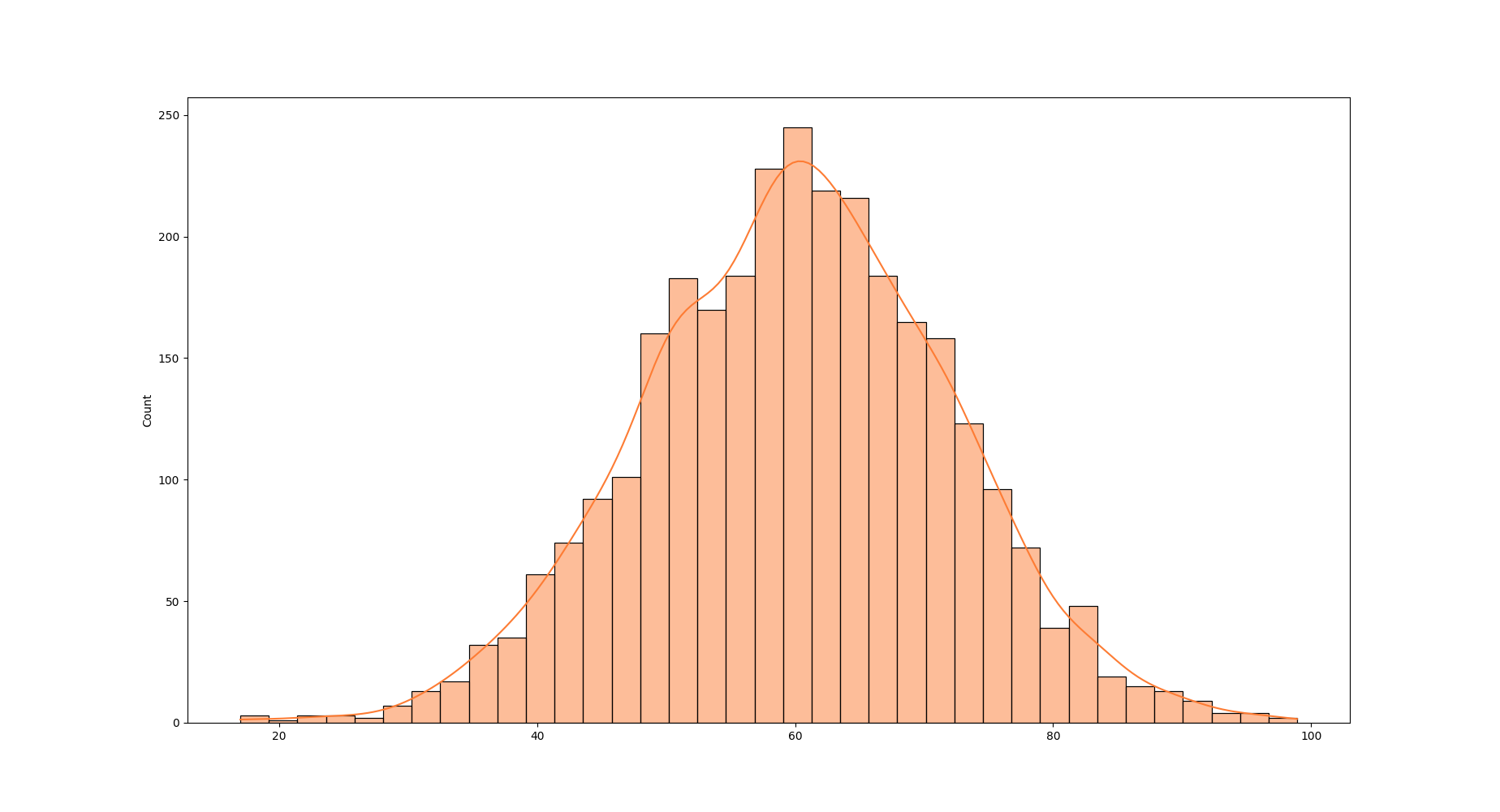
Weight distribution for some segment
Yet, if we just do that the naive way, this could happen :
ID |
age |
weight |
size |
job |
sport |
|---|---|---|---|---|---|
random 1233 |
82 |
12 |
193 |
Salarymen |
American Football |
(Note: of course retired women may play american football yet weighting 12kg and playing american football when you are 82 years old is quite odd)
There are too tarpit when generating fake data :
Assuming everything is a normal distribution and reducing a feature to its average and its deviation. In fact, most of real world distribution are skewed
not caring about joint probability distribution.
And this is were good synthetic Data Generator come to the rescue.
Performance of synthetic Data Generator evaluation
Like every datascience modelisation, synthetic data generation needs some metric to measure performance of different algorithm. This metrics should capture three expected output of synthetic data :
distribution should “looks like” real data
joint distribution too ( of course, someone who weight 12kj should not be 1,93m tall ) ( likelihood fitness )
Modelisation performance should stay the same ( machine learning efficiency )
Statistical properties of Generated Synthetic Data
First obvious way to generate synthetic data is assume every feature follows a normal distribution, compute means and deviation and generate data from gaussian distribution ( or discrete uniform distribution ) with the following statistics :
stats |
price |
bedrooms |
bathrooms |
sqft_living |
sqft_lot |
yr_built |
|---|---|---|---|---|---|---|
mean |
5.393670e+05 |
3.368912 |
1.747104 |
2078.563541 |
1.529471e+04 |
1971 |
std |
3.647895e+05 |
0.937394 |
0.735760 |
917 |
4.261295e+04 |
29 |
min |
7.500000e+04 |
0.000000 |
0.000000 |
290 |
5.200000e+02 |
1900 |
25% |
3.220000e+05 |
3.000000 |
1.000000 |
1430 |
5.060000e+03 |
1952 |
50% |
4.500000e+05 |
3.000000 |
2.000000 |
1910 |
7.639000e+03 |
1975 |
75% |
6.412250e+05 |
4.000000 |
2.000000 |
2550 |
1.075750e+04 |
1997 |
max |
7.062500e+06 |
33.000000 |
8.000000 |
13540 |
1.651359e+06 |
In python
[...]
nrm = pd.DataFrame()

for feat in ["price","sqft_living","sqft_lot","yr_built"]:
   stats=src.describe()[feat].astype(int)
   mu, sigma = stats['mean'], stats['std']
   s = np.random.normal(mu, sigma, len(dst))
   nrm[feat] = s.astype(int)

# For discrete Features
for feat in ["bedrooms","bathrooms"]:
   p_bath = (src.groupby(feat).count()/len(src))["price"]
   b=np.random.choice(p_bath.index, p=p_bath.values,size=len(dst))
   nrm[feat] = b
Yet this lead to bad feature distribution and joint distribution.
In the following plot, we show the distribution of features of a dataset (blue) , distribution of a synthetic dataset generated with a CTGAN in quick mode (orange, only 100 epoch for fitting ) and distribution of data assuming each feature is independant and follows a normal distrbution ( see code above )
For prices, we see that generated data perfectly captured the distribution of it, so good that we barely see the orange curve. Gaussian random data has same mean and deviation than original data but clearly does not fit the true data distribution. For yr_built, the synthetic data generator (orange) struggles to perfectly capture the true distribution (blue) but it looks better than the average
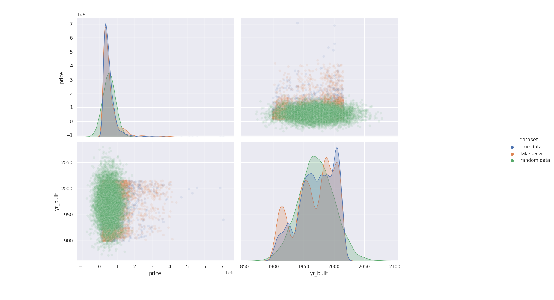
prices and bedrooms distribution
Here below is same density chart for prices, zoomed
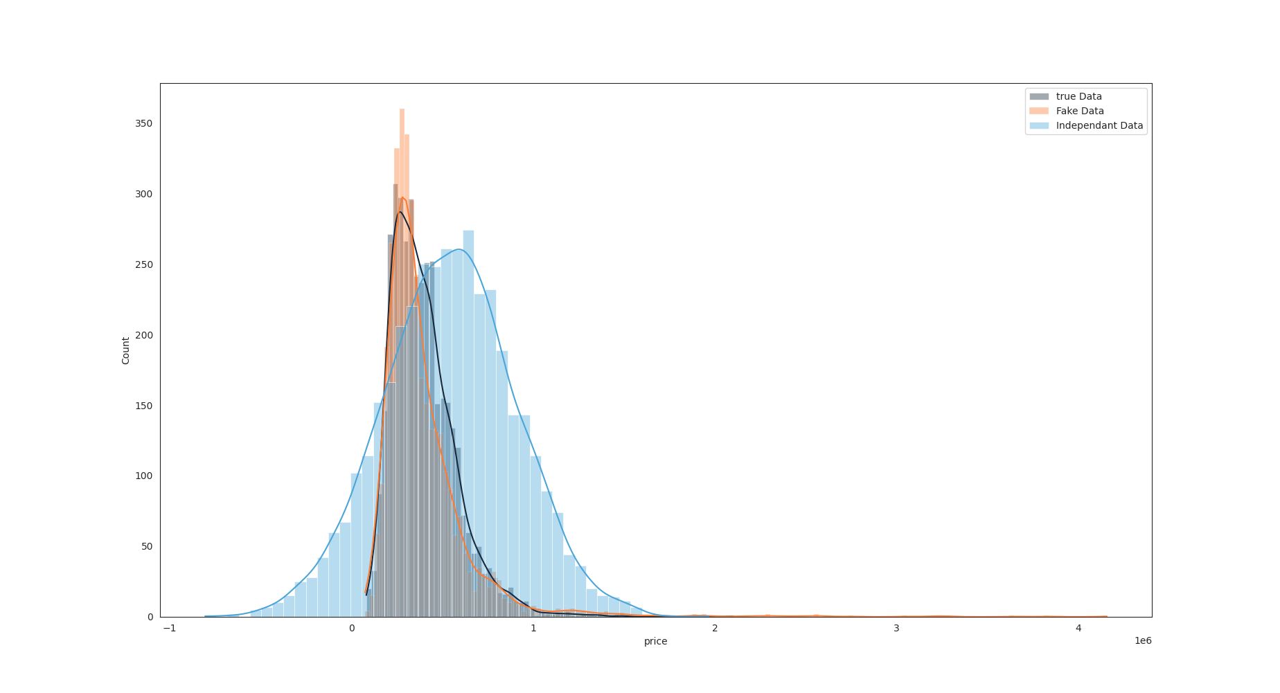
Zoom on price distribution
It’s more difficult to see joint distribution on this chart but we can draw contourmap to get a better view :
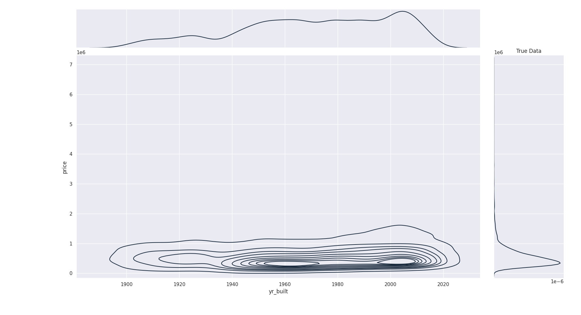
Original true Data Joint distribution of prices and year constructed
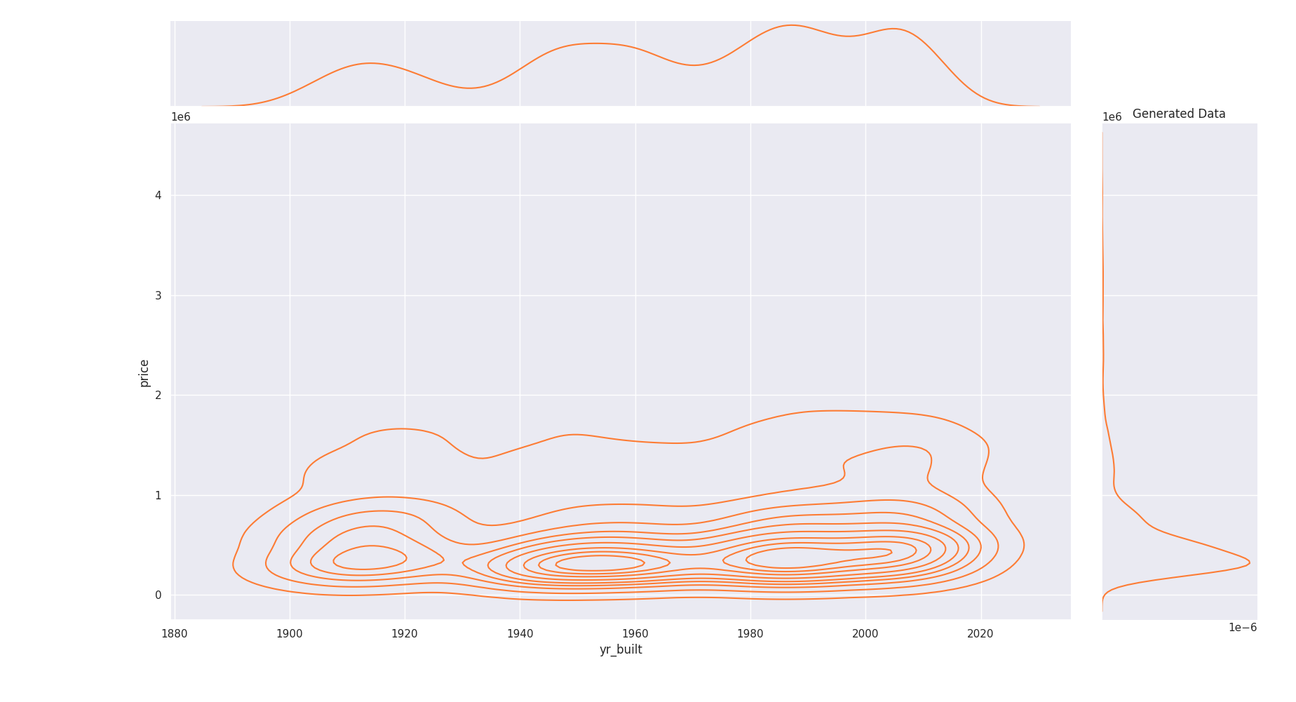
Generated Data Joint distribution of same features. We see density start to reach those of real data
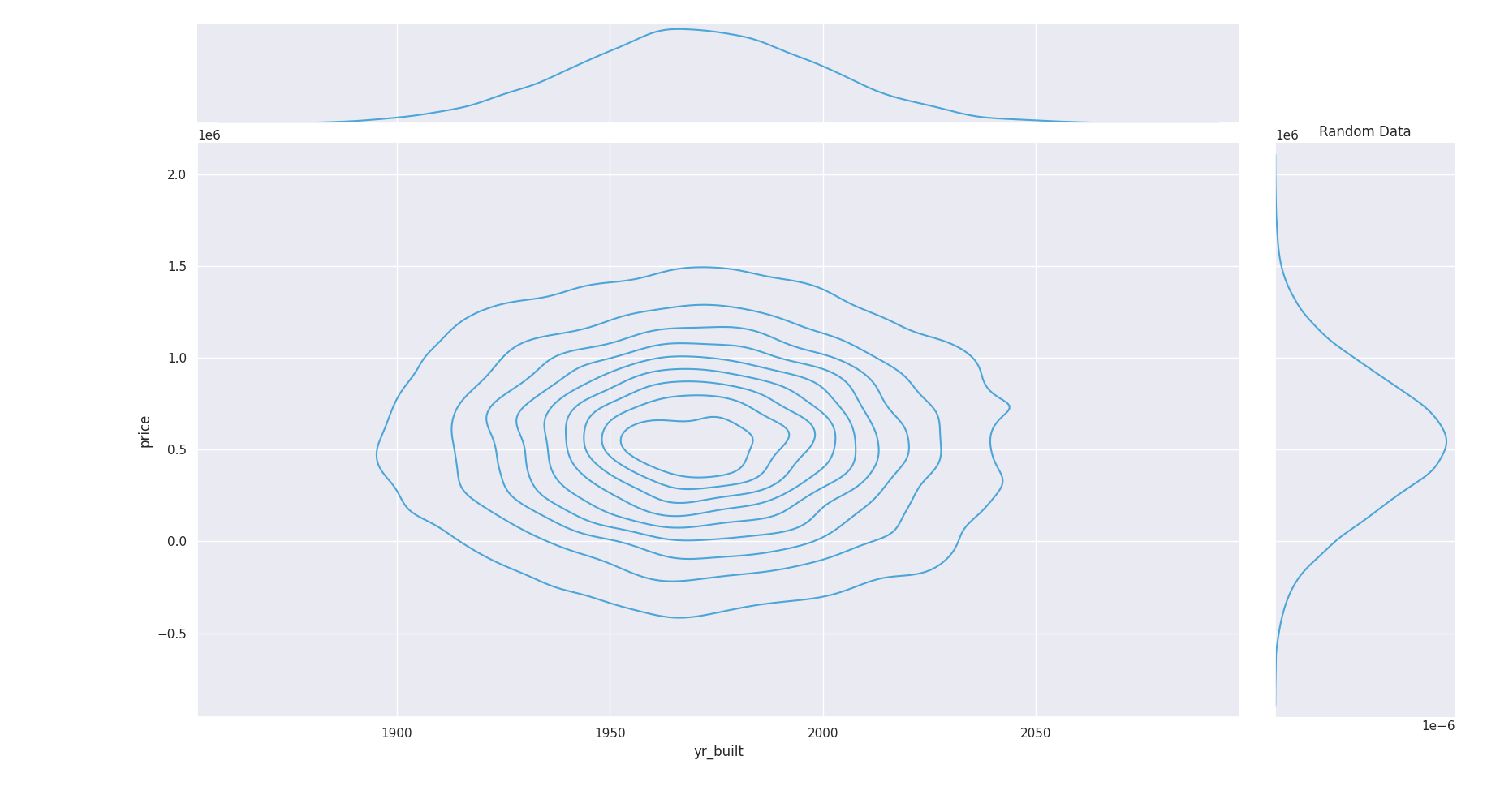
Independant random variable distribution : jointplot density is totally wrong
The same conclusion goes for others features too. Random independant data do not fit distribution and joint distribution as good as properly generated data :
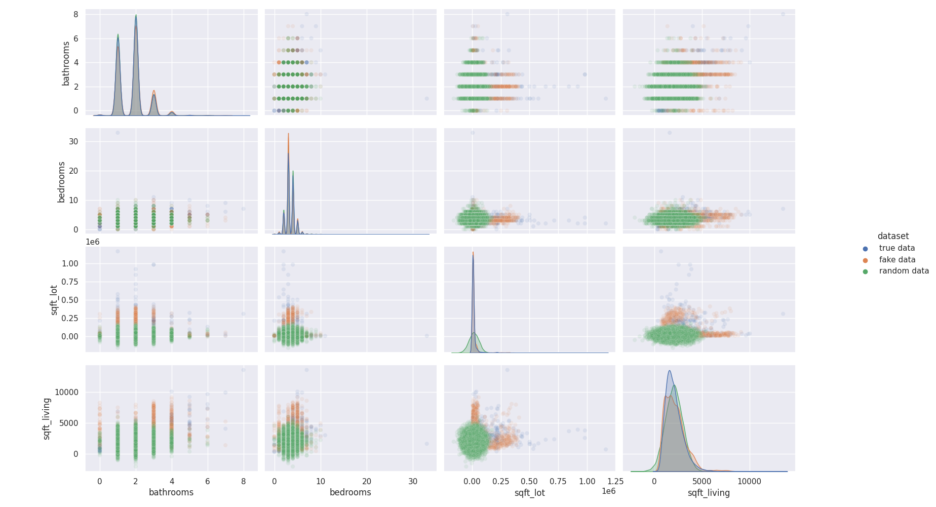
each feature has its own distribution and distribution relative to others
Of course, better models than simple Normal distribution exist. You can build kernel density estimation, gaussian mixture model or use other distribution thant a normal one yet doing so mean you start to use more and more complex model, till you ‘ll discover that going for Generative Adversarial Network is the way to go.
Generating good Synthetic Data
Like image before, Tabular data benefits from usage of Generative Adversarial Networks with Discriminator. In order to avoid the issue shown above, we can train a neural network on data whom input would be for each sampe a vector of :
discrete probability for each mode of categorical variable
probability of each mode of a a gaussian mixture model
The network is then tasked to generate a “fake sample” output and a Discriminator then try to guess if this output comes from the Generator or from the the true datas.
By doing this, the Generor will learn both distribution and joint distribution between each feature, converging to a generator that output sample “as true as the real one”.
The current best implementation of this idea is CTGAN that you can use on our Marketplace
Machine Learning efficiency
Of course, the best practical performance estimation of generated data is Machine Learning efficiency. We ran some performance test on our automl platform with the optimal parameters ( all models tried, hyperoptimisation and Blending of model ) on 3 datasets with the same target :
Original dataset
Synthetic dataset fitt on 800 epochs
random Dataset with no joint probability
We expect that by using automl platform, only data quality would change the performance.
Here are the results :
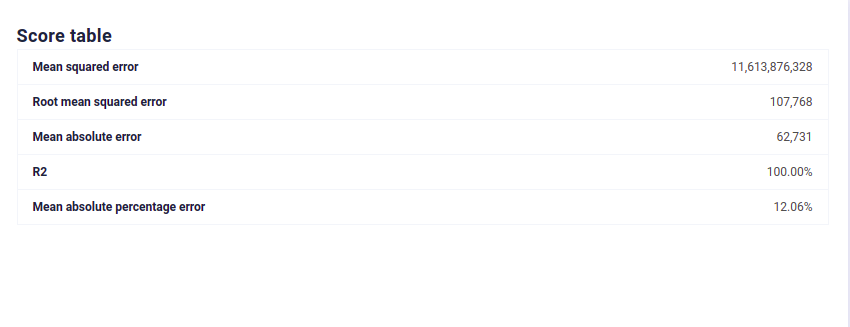
Modelisation on true Data
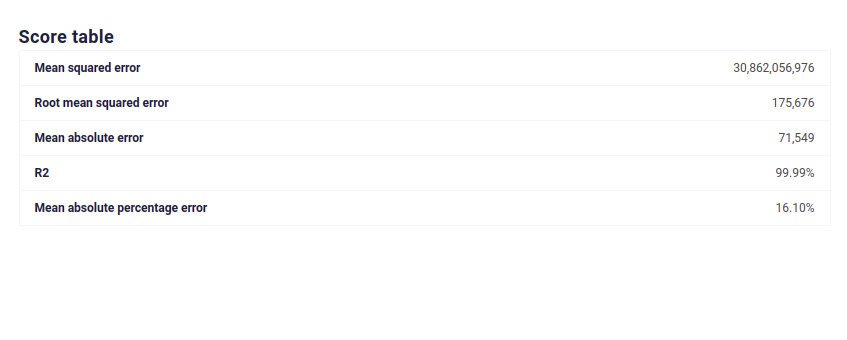
Modelisation on Synthetic Data
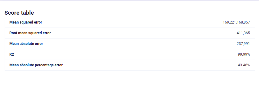
Modelisation on random independant data
We see that with CTGAN Synthetic Data, Machine Learning efficiency is preserved, which is not the case for independant data distribution. Moreover, this efficiency is good even for sgemnt of the original dataset, meaning you can generate synthetic samples for under represented category and keep their signal high enough to fix bias in your dataset.
Going Further
You can read the original paper for CTGAN and get it here.
The CTGAN implementation is available on our Marketplace and you can test it with one of our public standard Dataset
Remember that synthetic datas is very useful when you need to enforce data privacy or unbiase dataset. Training a Synthetic Data Generator for few hours build a generator that can be used to generate data in a few seconds and thus synthetic data should become part of your datascientist toolset too.